
by Kyle
Olszewski (kolszewski3 AT mail DOT gatech DOT edu)
Final Project
CS7490 – Image Synthesis
Professor Greg Turk
Introduction:
For my final project for CS7490: Advanced Image Synthesis, I implemented a distribution ray tracer. This ray tracer provides for effects such as anti-aliasing, soft shadows, diffuse reflections/refractions, and depth-of-field effects. To accelerate the performance of this ray tracer, I used spatial subdivision techniques to limit the total number of primitives which a given ray passing through the scene must intersect; I also implemented the ray tracer in parallel using multiple computers. Finally, I experimented with adding a motion blur effect, as well as using height field rendering techniques to add details to the surfaces of low resolution polygonal meshes. In the following sections, I will describe how these techniques work, discuss my implementation of the ray tracer, and show some example results.
Techniques:
Distribution Ray Tracing:
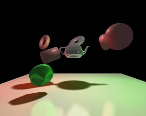
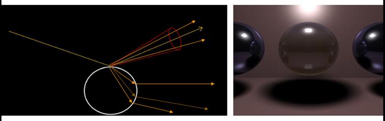
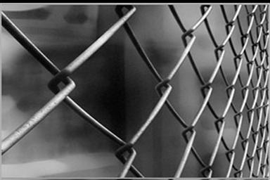
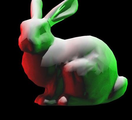
In brief, distribution ray tracing [6] techniques attempt to resolve some of the issues with conventional ray tracing techniques which ultimately cause the resulting images to have a very “computer generated” look to them. For example, a standard ray tracer will simply determine the color value of a given pixel by tracing a single ray from the center of projection through the center of the pixel, determining which object the ray interests first, and using the properties of this object (such as the material properties and orientation towards the light sources) to determine its resulting color value. As a result of using only this single ray per pixel, objects in the scene may suffer from aliasing, i.e., they may very jagged silhouettes due to the fact that the rays going through the center of some pixels may interest an object while the rays passing through the center of nearby pixels will just barely miss it. Casting a single reflection ray from the intersection point to determine what color value it reflects results in having objects which are all treated as mirrors, meaning that all of the objects will produce perfect reflections rather than the sort of glossy reflections seen in objects such as a dull spoon. Treating every light source as a point light source and casting a single shadow ray from an intersection point towards this point in order to determine if it is illuminated by this light source produces very sharp, “hard” shadows which do not produce the gradual transition from lit to occluded regions which are produced by area light sources. The result of using techniques such as these is images which look very artificial, such as the one seen below:
Distribution ray tracing
resolves the aforementioned issues and others by using
Soft shadows may be produced by treating each light source as an area light source, represented by a quadrilateral, which is divided into several sub-sections. From a given intersection point, a shadow ray is cast to each sub-section in order to determine whether the light from that section reaches the intersection point.
Casting rays to the same point in each sub-section causes the light source to be treated as multiple point sources, leading to the “banding” in the resulting shadows as seen below:
To resolve this, each ray samples a random point in its given sub-section; this gives us an approximation of the total amount of light reaching the surface from this light source, as seen below:
Diffuse reflections are created by tracing multiple reflection rays distributed over an interval around the “perfect” reflection vector and integrating the resulting color values. Thus, the reflected value at each point will be the average color value of each of these reflected rays. Using a wider interval results in “duller” reflections, while using a smaller interval results in sharper ones. By distributing multiple refraction rays around the “perfect” refraction vector, we can produce glossy refractions as well.
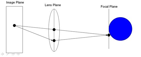
Finally, one can use distribution ray tracing techniques to add a “depth of field” effect to the image, allowing objects to lose focus as they move away from the focal plane, as they would in an image recorded using a real lens. Conventional ray tracing simply traces a ray from the center of projection through the center of each pixel in the image plane, resulting in images in which every object is in perfect focus.
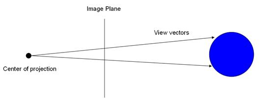
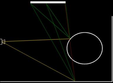
To implement the depth-of-field effect, one must simulate the effects of using a lens to record the image. To do this, we define a “lens plane” between the image plane and the “focal plane” in the scene at which every object should be in perfect focus. We create a ray passing from a given pixel on the image plane through the center point of this lens plane, determining the point on the focal plane which would be intersected by this ray. We then sample a random point on the “lens” (a random point on the lens plane within some distance of the center point of this plane, where this distance is determined by the “size” of the lens we use) and trace a ray from this point to the point on the focal plane intersected by the previous ray, as seen below:

Thus, when the object being intersected by this ray is exactly on the focal plane, this ray will intersect the same object as the ray passing through the center of the lens plane. The farther the object is from this plane, however, the distance between the intersection points of the rays increases. When enough samples are used, this results in images in which the objects close to the focal plane are in perfect focus, while objects not on this plane will lose focus as they move farther and farther away from this plane.
To avoid having to use an extremely large number of rays, one can use rays which sample in multiple dimensions. For example, instead of having the ray through each sub-pixel spawn multiple shadow rays, each sub-pixel ray can spawn a single shadow ray which samples a different sub-section of the area light source. This gives us acceptable results in a much shorter amount of time. However, even using these techniques, a large number of rays is still required; for example, to render a 1000x1000 pixel scene using 16 sub-pixel samples requires 16 million primary rays alone, rather than the 1 million needed for conventional ray tracing. Thus, in the following section, I will discuss how I used spatial subdivision techniques to limit the total amount of ray-primitive intersections needed to trace a give ray through the scene.
Spatial Subdivision:
I implemented the spatial subdivision scheme in this renderer using KD-trees. In brief, KD-Trees are a special case of binary space partitioning trees (BSPs). In BSPs, at each node we choose a split plane which divides the objects in that node into two different areas, thus creating two child nodes for that node. In KD-trees, we have the requirement that each split plane must be perpendicular to one of the coordinate system axes. Thus, for a 3-dimensional space, we may subdivide the scene by first choosing a split plane which is perpendicular to the x axis; then at the next level, we choose a split plane which is perpendicular to the y-axis; and at the next level the split plane is perpendicular to the z-axis. We iterate through the coordinate system axes, thereby creating nodes which are not extremely wide in any particular dimension, as seen below:
The primitives in the objects in the scene may be stored in the leaf nodes of the tree. We repeat this subdivision process until we reach some termination criteria; for my renderer, I chose to terminate when the nodes in the tree were at depth 20, or when there were less than 10 primitives in a given node.
The efficiency of traversing a KD-tree is determined by the heuristic used to find the split plane at each node of the tree. The naïve method for doing so would be to create balanced trees, in which there are an equal number of primitives in each leaf node, as seen below:
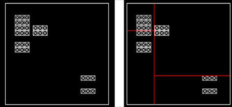
While fast to construct and easy to implement, such trees are not ideal for ray tracing programs. The problem is that rays passing through the scene will never pass through an empty leaf node; for each leaf node it intersects, the ray will have to perform some intersection tests regardless of how close it is to the objects stored in that node. Picture a ray passing from the bottom left to the top right of the previous image; since that ray only passes through empty space, we would like to have a tree such that the ray does not perform any intersection tests, allowing it to travel “for free” through such large empty spaces.
Thus, we would rather use a heuristic which allows us to create trees in which the primitives in the objects in the scene are stored in nodes representing very small portions of the scene, thus isolating them from the very large empty spaces in the scene, as seen below:
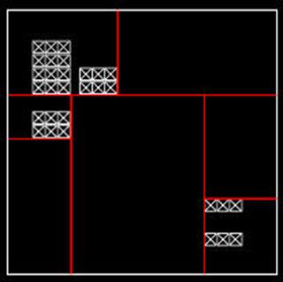
This allows a ray which does not come extremely close to some set of primitives to avoid having to perform intersection tests with them, thus letting it quickly traverse the empty spaces in the tree. To construct such as tree, we use what is known as the “Surface Area Heuristic,” or SAH. The idea of this heuristic is that the probability of a ray intersecting a given node in the tree is roughly related to its surface area:
area = 2 (height * width + height * depth + width*depth)
Nodes with more surface area are more likely to be intersected than nodes with relatively little surface area. Thus, we approximate the “cost” of traversing a given node using the formula:
cost = Costtraversal + area * prims * Costintersect
where Costraversal is the cost of checking to see if the ray enters the node, prims is the number of primitives in the node, and Costintersect is the cost of performing an intersection test for a single primitive.
To determine the “cost” of a given split plane position, we simply find the number of primitives on each side of the split plane, determine the “cost” of each resulting child node using the formula above, and add the resulting costs. When choosing from multiple candidate split plane positions, we simply select the split plane position with the minimal cost. We could thus find the optimal split plane position by performing this test at the “left” and “right” boundary position of each primitive in the scene (where “left” and “right” refer to the greatest and least values of the vertices in this primitive in the dimension in which we are choosing the split plane position for this node of the tree). However, for scenes with a very large number of primitives, this may take an extremely long time. A faster method is to choose a constant number of candidate split positions spaced at regular intervals in the space contained within the node, performing the test to determine the “cost” of each candidate position, and choosing the split position with the minimal cost. With a small enough sampling interval, the resulting split plane position is a close approximation of the optimal split plane position. In my renderer, I performed this test at 32 regular intervals in each node. The resulting Kd-tree construction process took an average of roughly 12 seconds for a scene with roughly 10,100 primitives.
Once we have constructed the KD-tree, traversing it during the ray tracing process is a relatively simple process. We may represent any point K on a ray as the sum of P, the origin point of the ray, and u*V, where V is the direction vector of the ray and u is a scalar value indicating the distance along this ray from the origin point P:
K = P + u*V
We know P and V for each ray passing through the scene; if we know one of the values (x,y,z) for K, we may use this value to find the u value for K, which tells us how far along the ray this point is.
u = (K-P)/V
Since the split planes of each node of the KD tree are all axis-aligned, we know the value of either the x,y, or z position for the split plane of each node as well as the planes which create a bounding box around the area within the node . Thus, one a ray has entered a given node of the tree, we may determine which child nodes it passes through using a relatively simple test. By plugging the known coordinate positions for the split plane and for each of the bounding box planes into the formula above, we may determine the u values which tell use how far along the ray the points are at which the ray enters the node, exits the node, and intersects the split plane in the node, as seen below:
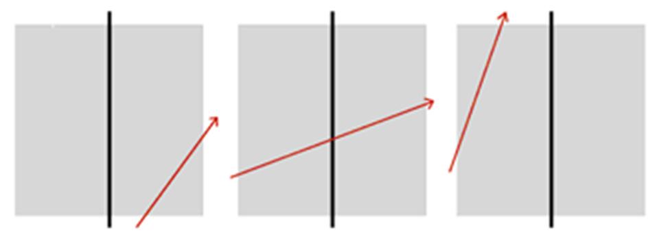
By comparing the coordinate position at which the ray enters the node with the coordinate position of the split plane, we may determine whether it first passes through the “left” or “right” child node. Then, we compare the u values for the entry point, exit point, and split plane intersection point. If the ray intersects the split plane before or after it enters the node (meaning that the u value of the split plane intersection position is less than the u value of the entry point or greater than the u value of the exit point), as seen in the first and third images above, we know that it simply passes through the first child node it intersects within this node. If the ray enters the node, intersects the split plane position, and then exits the node (meaning that the u value of the split plane intersection point is between the u values of the entry and exit points), as seen in the second image above, we know that the ray traverses both the left and right child nodes, so we must repeat this test at each one. This process repeats until we reach a leaf node, at which point we perform the intersection tests with the primitives in this node.
Using these techniques, I was able to achieve a great reduction in the total number of ray-primitive intersection tests used in my renderer (see “Results” below), leading to a large reduction in the amount of time required to render a given scene.
Motion Blur:
One can implement motion blur using distribution ray tracing techniques by giving every object a direction vector and speed; the rays traced through the scene can them sample a random point in time, and be intersected with the primitives at their position at that point in time. The result is “blurred” images which resemble images which are recorded with a camera with a relatively low shutter speed.
Unfortunately, using this spatial subdivision technique makes implementing motion blur effects using distribution ray tracing techniques quite difficult. This is due to the fact that these trees treat every object as having a static position in the scene. Thus, one cannot use the tree with scenes in which objects may have any position along their direction vector. Thus, to implement motion blur using my renderer, I instead gave the camera a direction vector; with each sample ray, I generated a random value and displaced the camera position along this vector according to the randomly generated value. The result is a motion blur effect in which every object in the scene is blurred, as it would be if a camera was moved relative to the scene it is recording. This means that this technique can not be used to blur moving objects against a static background. The result of using this technique is pictured below.
Height field rendering:
For the height field rendering aspect of this project, I created a CPU-level implementation of the GPU shader techniques described in “Dynamic Parallax Occlusion Mapping with Approximate Soft Shadows” [7]. In essence, these techniques rely on a tangent-space ray tracing scheme. Here “tangent-space” refers to a coordinate system defined relative to the surface of a given object. We may traverse this coordinate system using the (u,v) texture coordinates along the surface of this object, as well as another value which indicates the height of a point relative to the object surface. To define this coordinate system for a given point on the object, we need 3 orthogonal unit vectors: the standard normal vector, which points out from the surface of the object; the tangent vector, which points in the direction of increasing u values for the texture coordinates on the surface of the object; and the bi-normal vector, which points in the direction of the increasing v values in the texture coordinates along the surface of the object.
Using these 3 vectors, we may transform a world-space view vector into the tangent-space coordinate system. The (u,v) texture coordinates at the intersection point of the view vector with the object tell us the “starting position,” at which the tangent-space view ray is at a height of 0 in the tangent-space of the object.
We then trace this ray through the tangent space of the object in order to determine the intersection point of the view ray with the object surface, which is displaced from the surface of the bounding polygonal mesh. To do this, we store a “height field” in one of the channels of a texture map we apply to this surface. The values of this height field tell us the displaced positions of each of the points on the object surface, which are extruded downwards from the polygonal mesh of the object. Thus 0 represents a height value which is not displaced at all, meaning that this point on the object surface is on the polygonal mesh which bounds the displaced surface of the object; while 1 represents a point which is extruded downwards to the maximum possible amount.
To trace a ray through this tangent space, we sample several regular intervals along the view ray, finding the height value of the ray at each sampling position and using the texture coordinates at the corresponding point on the object surface to find the height value of this displaced point on the object. We compare these values; when the height of the view ray is below the height value of a point on the object, we know that we have found a point at which the view ray has gone below the displaced surface of the object. We use the height value of the ray and the sampled height field value at this position with the ray height and height field values from the previous sampling point in order to determine the exact texture coordinate position at which the view ray intersects the surface of the object. This basic tangent-space ray tracing scheme is illustrated below:
Using the texture coordinates of the intersection point, we may find the color and normal values for the displaced surface of the object. Using these values allows us to create an illusion of depth and complexity on relatively low-resolution polygonal meshes, such as a cube (see “Results” below).
(Note: The above description provides only a rough description of the algorithm used for this implementation. See [7] for more details.)
Unfortunately, due to the fact that these techniques required me to use a ray-tracing scheme on top of my original ray-tracer (and that I did not have access to the vectorized operations available on the GPU, which was the intended platform for these techniques), the performance when using these techniques is extremely slow. I thus implemented this technique in a second version of this project, in which these techniques are implemented on a single face of a cube, and compared to the results from using standard normal and texture mapping on the other faces. Both implementations of the project may be found in “Software” below.
My Implementation:
I implemented this program in C++, using a conventional ray tracer I had written as an undergraduate as a template. Parameters such as light and camera positions and orientations are represented in a data file which is loaded into the program before the ray-tracing begins. The objects in the scene are represented as triangle meshes, which are loaded from an .obj file representing the scene.
I performed this project in conjunction with a project in CS6230: High Performance Parallel Computing. As a result I had access to 10 nodes of the Warp cluster at Georgia Tech. Each node has 2 dual-core 3.2 GHz CPUs, meaning that I could have up to 40 processes running in parallel (although in practice the renderer received little benefit from using more than 20 processes). In my program, one process acts as a “leader,” dividing the scene up into 16 x 16 tiles and sending messages to each of the other processes telling them which tiles to render. The other processes render these tiles and send their results back to the leader process; the leader process stores the results in an image buffer and sends another tile to the responding process. This repeats until all of the tiles have been rendered, at which point the image buffer is written to a .ppm image file. I used the Warp cluster’s implementation of the Message Passing Interface (MPI) to parallelize this program. The speedup from running this program in parallel is described in the following section.
Results:
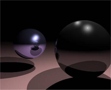
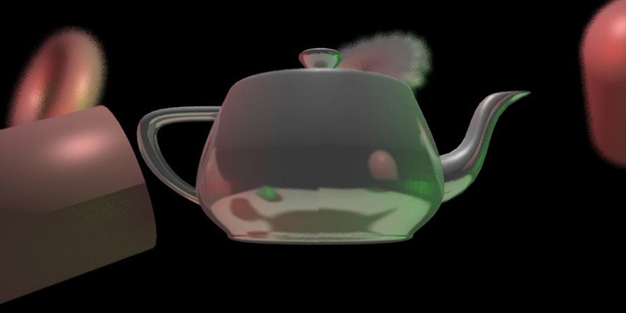
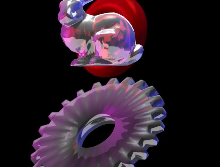
Below are 2 sample images rendered using the distribution ray tracing and spatial subdivision techniques described above. Note the soft shadows and diffuse reflections on the box on the bottom of the images:
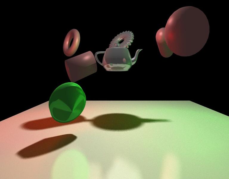
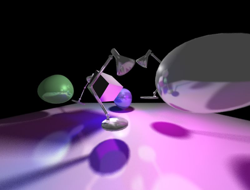
Here are some details about these images:
First Image:
– 1000x800 pixels
– ~10,100 polygons
– Approximately 18.5 billion intersection tests required
– 32 samples for anti-aliasing/DOF; primary rays each spawn 1 shadow ray sample, 8 reflection ray samples
– Rendered in 5210 seconds using 1 process; rendered in 320 seconds using 20 processes
Second Image:
– 800x600 pixels
– ~5,500 polygons
– Approximately 16 billion intersection tests required
– 32 samples for anti-aliasing/DOF; primary rays each spawn 1 shadow ray sample 8 reflection ray samples, 8 refraction ray samples
– Rendered in 8240 seconds using 1 process; rendered in 610 seconds using 20 processes.
Note the total number of intersection tests required to render each scene. Using a naïve approach, intersecting each of the roughly 32,000,000 primary rays in the first image with each of the 10,000 primitives in the scene would require roughly 320,000,000,000 intersection tests; using spatial subdivision, however, we only need a total of roughly 1/20th of this number of intersection tests for all of the rays in the scene!
Here are some examples of specific effects supported by this renderer:
Anti-aliasing:
Diffuse Reflections/Depth of Field:
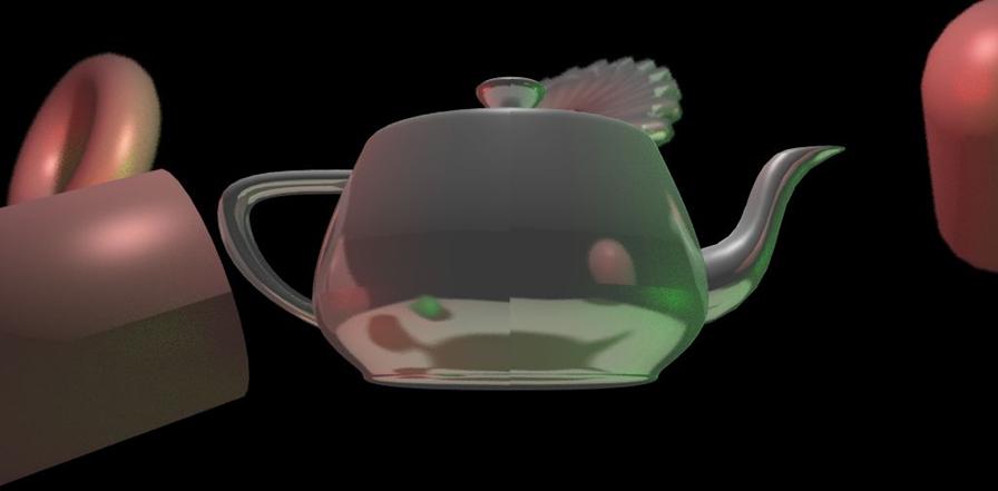
Diffuse Refractions:
Height Field rendering:
Here are some sample images of the results from my height field rendering techniques from the second version of the program. The left image simply uses standard texture and normal mapping. The right image uses height field rendering techniques on the lower right face. Notice how these techniques add an illusion of depth and complexity to the cube’s face (which consists of only 2 triangle primitives).
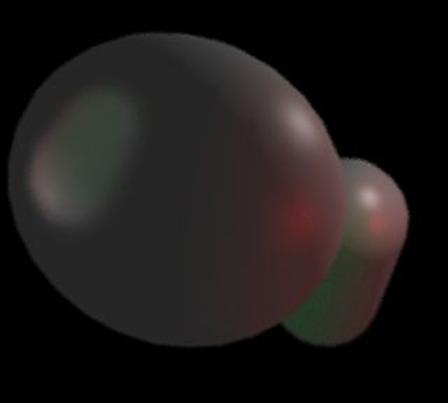
Motion blur:
Here are the results from shifting the camera position along a direction vector based on a randomly sampled time value:
Here are a few other example images rendered while testing my program:
Software:
The following .zip files contain the software for this project. The first version can be used to render the first 2 example scenes seen above, following the instructions in the README file:
The second version can be used to render the images above implementing the height field rendering and motion blur techniques seen above, again following the README file instructions:
Note that these programs were meant to be compiled and executed on the Warp cluster at Georgia Tech.
References:
[1] Woo, A. Ray Tracing Polygons Using Spatial Subdivision.
(http://portal.acm.org/citation.cfm?coll=GUIDE&dl=GUIDE&id=155316)
[2] Wald,
[3] Bikker, J. Raytracing: Theory and Implementation.
(http://www.devmaster.net/articles/raytracing_series/part1.php)
[4] Bigler, J., Stephens, A., Parker, S. Design for Parallel Interactive Ray Tracing Systems.
(http://www.sci.utah.edu/~abe/rt06/manta-rt06.pdf)
[5] Stone, J.E. An Efficient Library for Parallel Ray Tracing and Animation.
(http://jedi.ks.uiuc.edu/~johns/raytracer/papers/thesis.pdf)
[6] Cook, R. Distribution Ray Tracing. (http://portal.acm.org/citation.cfm?id=808590)
[7] Tatarchuk, N. 2006. “Dynamic Parallax Occlusion Mapping with Approximate Soft Shadows.” (http://portal.acm.org/citation.cfm?id=1111423)